Chapter 5 Models for nonideal flow
The information provided by RTD functions is essential to know if a reactor has dead zones or bypassing. These situations affect the reactor performance. Thus, the main target is answering the question “How much bypassing or dead volume is acceptable?”.
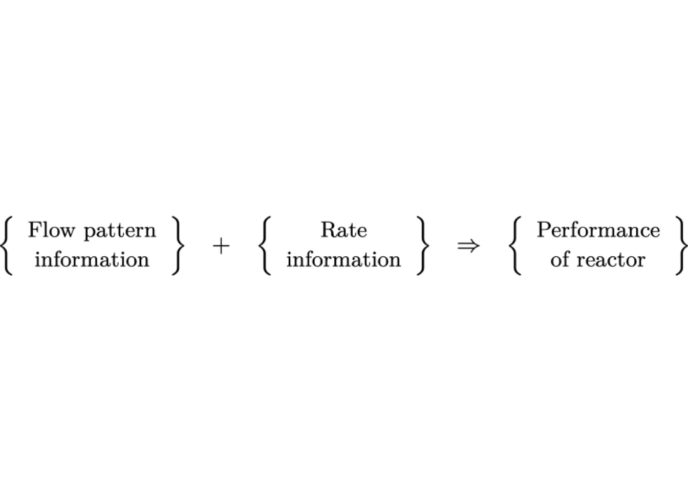
For answering, the chemical engineer needs to calculate the performance of the reactor. Furthermore, to do so, two types of information are required: the flow patterns and the kinetic model.
The information provided by RTD functions is essential to know if a reactor has dead zones or bypassing. These situations affect the reactor performance. Thus, the main target is answering the question “How much bypassing or dead volume is acceptable?’’.
For answering, the chemical engineer needs to calculate the performance of the reactor. Furthermore, to do so, two types of information are required: the flow patterns and the kinetic model.
The RTD curves found from tracer studies are only partial information on the details of the flow patterns because all that is known is the length of time-specific fractions of the fluid stay in the vessel (macromixing), but neither what of these fractions do while in the vessel nor in what geometric locations they reside, that is, information on micromixing.
As a result, several mathematical models of reactor performance have been developed to estimate the conversion levels in a nonideal reactor. (C. Jr. Hill 1977)
The micromixing behavior has two extremes views:
- Complete segregation: any fluid element is isolated from all other fluid elements and retains its identity throughout the entire vessel. No micromixing occurs, but macromixing may occur.
- Complete dispersion: fluid elements interact and mix thoroughly at the microscopic level.
Besides the degree of segregation of fluid elements, another aspect of mixing is the relative time in passage through a vessel at which fluid element mix (‘’earliness’’ of mixing). (Missen, Mims, and Bradley 1999)
In general, a mathematical model for nonideal flow in a vessel provides a characterization of mixing and flow behavior. Although it may appear to be an independent alternative to the experimental measurement of RTD, the latter may be required to determine the parameter(s) of the model.
For that reason, these mathematical models can be classified in function of the number of adjustable parameters. (Fogler 2008)
- Zero adjustable parameters
- segregation model
- maximum mixedness model
- One parameter model
- tanks-in-series model
- dispersion model
- Two adjustable parameters
- actual reactor modeled as combinations of ideal reactors
These parameters are correlated as functions of fluid and flow properties, reactor configurations, along with other vital features, and can be used in design calculations.
Generally speaking, the more adjustable parameters used in a model, the better the correlation between predicted and observed RTD would be. These adjustable parameters are often related to RTD moments and are usually expressed in terms of dimensionless moments about the mean.
The usual approach is developing a model flow system with the same RTD as the existing system. Provided that the conservation equations can be written for this model system, the performance of the actual vessel can be predicted.
5.1 Zero adjustable parameters
Segregational or macrofluid model
This model represents the micromixing condition of complete segregation (no mixing) of fluid elements, which means that fluid flows through a vessel with no mixing between adjacent fluid elements. The feed enters the reactor as little packets of fluid. Each packet retains its identity as they pass through the vessel; there is no mass exchange between individual packets. However, packets can mix each other in the reactor. Thus those that enter at some time, t, will not all leave at the same time.
Each packet can be treated as a small ideal batch reactor. A reaction (or reactions) takes place as the tiny packets move through the vessel. The composition of each packet changes while it is flowing through the vessel. However, its final conversion will depend on how long the packet has spent in the vessel. (Roberts 2009).
After leaving the reactor, all fluid packets are mixed on a molecular level, and the average composition is measured. This situation is represented in Figure 5.1. (Roberts 2009)
![Segregational model scheme. [@roberts2009]](ebook_notes_5314_files/figure-html/fig004010c-1.png)
Figure 5.1: Segregational model scheme. (Roberts 2009)
When the packets are admitted to a CSTR, we can envisage two scenarios that involve perfect mixing: one with perfect mixing at the macroscale and the other with perfect mixing at the microscale, as is shown in Figure 5.2
![Different levels of mixing in a CSTR: (a) Segregational model, (b) Ideal CSTR model. [@hayes2013]](ebook_notes_5314_files/figure-html/fig004010d-1.png)
Figure 5.2: Different levels of mixing in a CSTR: (a) Segregational model, (b) Ideal CSTR model. (Hayes and Mmbaga 2013)
The conversion in a segregated tank reactor can be calculated using the ideal batch reactor equation design and the RTD curve. Each batch reactor has its conversion, which depends on its time in the tank. While the RTD gives information about the mean residence time.
The initial concentration of reactants in the packet is the same as the inlet concentration of the reactor. While each fluid element (assuming constant density) behaves as a batch reactor, the total reactor conversion is the average conversion of all the fluid elements at the outlet conditions. That is:
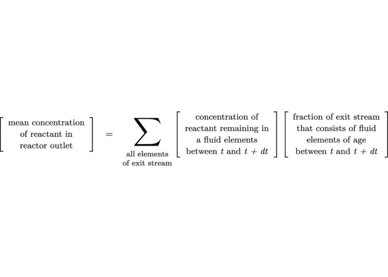
where the summation is over all fluid elements in the reactor exit stream. This equation can be written analytically as:
\[\begin{equation} \overline{C}_A = \int_0^\infty{C_A(\overline{t})\,\mathbf{E}(t)\,d\overline{t}} \tag{5.1} \end{equation}\]
Where \(C_A(t)\) depends on the residence time of the element.
\[\begin{equation*} \frac{d\,C_A(t)}{dt} = - r_A = k\,C_A(t) \end{equation*}\]
The equation (5.1) is rewritten as
\[\begin{equation} \frac{\overline{C}_A}{C_{A0}} = \int_0^\infty{\left(\frac{C_A(\overline{t})}{C_{A0}}\right)\,\mathbf{E}(t)\,d\,t} \approx \sum_{\substack{\text{\footnotesize{all age}}\\\text{\footnotesize{intervals}}}}\left(\frac{C_A}{C_{A0}}\right)\,\mathbf{E}(t)\,\Delta t \end{equation}\] \tag{5.2} or in terms of conversions \[\begin{equation} \overline{X}_A = \int_0^\infty{{\left(X_A(t)\right)}_\text{\footnotesize{element}}\,\mathbf{E}(t)\,dt} \tag{5.3} \end{equation}\]
Introducing the \(\mathbf{E}(t)\) curve for CSTR, Equation (5.2) becomes, \[\begin{equation*} \frac{\overline{C}_A}{C_{A0}} = \frac{1}{\overline{t}} \int_0^\infty{ \text{e}^{-k\,t}\,\text{e}^{-t/\overline{t}}\,d\,t} = \frac{1}{1 + k\,t} \end{equation*}\]
Now, introducing the \(\mathbf{E}(t)\) curve for a PFR, \[\begin{equation*} \frac{\overline{C}_A}{C_{A0}} = \frac{1}{\overline{t}} \int_0^\infty{ \text{e}^{-k\,t}\,\delta \left(t - \overline{t}\right)\,d\,t} = \text{e}^{-k\,\overline{t}} \end{equation*}\]
The methodology described above can be used without any flow pattern models at all, in that experimental concentration as a function of residence time and the measured RTD can be directly numerically integrated to predict the conversion in the flow reactor.
The segregational o macrofluid model is essential because it permits reactor behavior to be estimated directly from RTD, \(\mathbf{E}(t)\), and the reaction kinetics. No other information is necessary.
However, it is only strictly applicable to isothermal, single-phase systems. Extensions to more complicated behaviors are not straightforward. Therefore, other techniques are required for more general predictive and design purposes.
When we dealt with ideal reactors in series, we learned that:
- If the order of the reaction is greater than 1 \(\left(n > 1\right)\), we must keep the reactant concentration as high as possible for as long as possible to maximize fractional conversion. In order words, we must avoid mixing as long as possible. For example, the optimum arrangement will be a PFR first, then a small CSTR, and a large CSTR.
- If the order of the reaction is less than 1 \(\left(n < 1\right)\), we must drop the reactant concentration as low as possible, which means mix as soon as possible.
- Finally, if the order of the reaction is equal to 1, the order of reactors will not affect the final conversion.
The macrofluid model represents the latest possible mixing for a given RTD because there is no mixing between fluid elements until the reaction is over. For a reaction with an effective order greater than 1, the macrofluid model represents the best possible situation. It provides an upper bound on conversion. (Roberts 2009)
Conversely, for a reaction with a practical order of less than 1, the macrofluid model represents the possible situation. It provides a lower bound on conversion. In summary,
| Reaction order | Segregational model provide |
|---|---|
| \(>1\) | Upper bound of conversion |
| \(=1\) | Exact result |
| \(<1\) | Lower bound of conversion |
Exercise 5.1 (Calculation of conversion based on RTD) Calculate conversion for a reaction \[\begin{equation*} A \rightarrow B \end{equation*}\]
for a given RTD and segregation model.
| t (min) | c (g/m\(^3\)) | t (min) | c (g/m\(^3\)) |
|---|---|---|---|
| 1 | 1 | 7 | 4 |
| 2 | 3 | 8 | 3 |
| 3 | 8 | 9 | 2.2 |
| 4 | 10 | 10 | 1.5 |
| 5 | 8 | 12 | 0.6 |
| 6 | 6 | 14 | 0 |
\[\begin{equation*} r_A = - k\,C_A; \quad k = 0.1 \text{ min}^{-1} \end{equation*}\]
Solution
The solution in a Python script is available at link.
From data problem, the RTD is shown on the left size of Figure 5.3
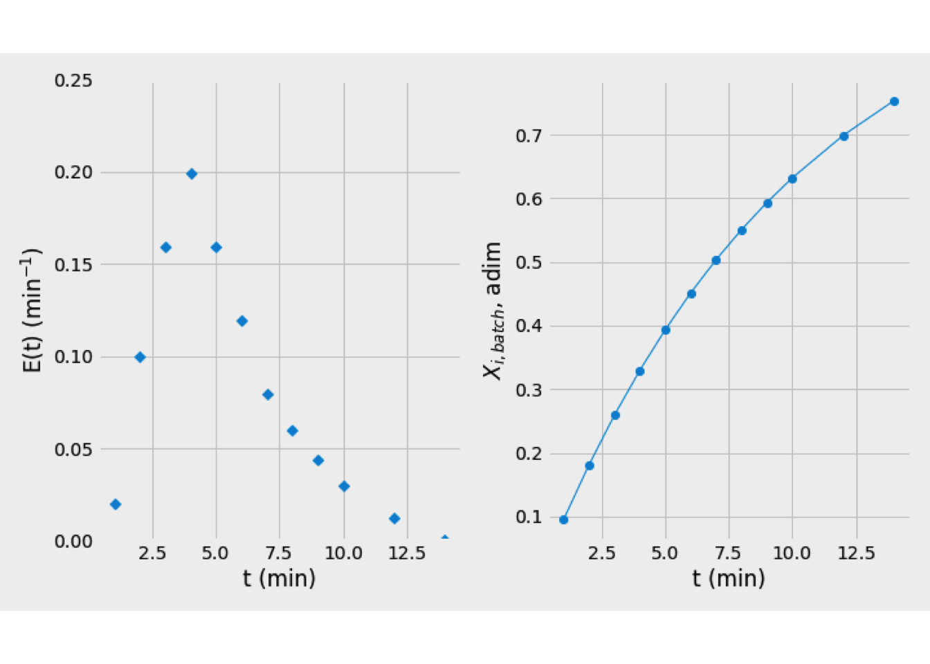
Figure 5.3: Graphical solution for the problem. Left: E(t) curve, Right: Fractional conversion curve.
From kinetic data, the fractional conversion for each batch reactor is \[\begin{equation*} X_{i,\text{batch}}(t) = 1 - \exp(-k\,t) \end{equation*}\] The profile of conversion is plotted right size of Figure 5.3
Finally, the mean conversion is estimated by Eq. (5.3) \[\begin{equation*} \overline{X}_i = \int_0^\infty {\left[1 - \exp(-k\,t) \right]\,\mathbf{E}(t)\,dt} = 0.3871 \end{equation*}\]
Maximum Mixedness Model (MMM)
The MMM for a reactor represents the micromixing condition of complete dispersion, where fluid elements are entirely mixed at the molecular level, which is the opposite extreme of the segregational model.
The MMM considers that the fluid packages of different residence times are mixed as early as possible in the flow system consistent with the observed RTD. For this reason, this model is also called Early mixing model.
This behavior can be modeled using a PFR with inlet side streams, as shown in Figure 5.4. The feed flow rate is distributed among the side streams in such a way as to match the required RTD function. It can be seen that in this arrangement, fluid entering the reactor in a given side stream, which has a residence time of zero, will mix radially with the fluid already present in the reactor completely.
![Scheme for modeling of maximum mixedness model. [@hayes2013]](ebook_notes_5314_files/figure-html/fig004010e-1.png)
Figure 5.4: Scheme for modeling of maximum mixedness model. (Hayes and Mmbaga 2013)
The conversion in a MM model can be calculated by performing a mole balance that considers all side streams. First, it is necessary to define an alternative variable, \(\lambda\), defined as the residence time remaining for an entering particle. All particles at a given \(\lambda\) have the same time left in the reactor but may have different ages.
![Control volume used to develop the mole balance for the maximum mixedness. [@hayes2013]](ebook_notes_5314_files/figure-html/fig004010f-1.png)
Figure 5.5: Control volume used to develop the mole balance for the maximum mixedness. (Hayes and Mmbaga 2013)
The concentration at the reactor outlet can be derived from mole balance equation. Take a small control volume of the reactor, as show in Figure 5.5. The mole balance over the discrete volumen element is \[\begin{equation} q\,C_A\left(\lambda + \Delta \lambda\right) + \Delta q\,C_{A0} + \Delta V \, r_A = \left( q + \Delta q \right)\,C_A (\lambda) \tag{5.4} \end{equation}\]
The volumetric flow rate at \(\lambda\) is the inlet volumetric flow, \(q\), plus the inlet side streams, \(\Delta q\), thus \[\begin{align*} \Delta q &= \upsilon_0 \, \mathbf{E}(\lambda) \, \Delta \lambda \\ q(\lambda) &= q(\lambda + \Delta \lambda) + \upsilon_0 \, \mathbf{E}(\lambda) \, \Delta \lambda \end{align*}\] where \(\upsilon_0\) is the total inlet volumetric flow rate fed to the reactor.
Rewriting \[\begin{equation} \frac{d\,q(\lambda)}{d\lambda} = - \upsilon_0\,\mathbf{E}(\lambda) \tag{5.5} \end{equation}\]
The inlet volumetric flow rate, \(\upsilon_0\) at the inlet of the reactor \((X_A = 0)\) is equal to zero because the fluid is fed only for side streams. Thus, integrating equation (5.5) considering that \(q(\lambda) = 0\) at \(\lambda = \infty\) and \(q(\lambda) = q(\lambda)\) at \(\lambda = \lambda\),
\[\begin{equation} \boxed{q(\lambda) = \upsilon_0\, \int_\lambda^\infty \mathbf{E}(\lambda)\,d\lambda = \upsilon_0 \left[1 - \mathbf{F}(\lambda)\right]} \tag{5.6} \end{equation}\] where \(q(\lambda)\) refers to volumetric flow rate inside the reactor at \(\lambda\)
The volume of fluid with a life expectancy between \(\lambda\) and \(\lambda + \Delta \lambda\) is \[\begin{equation} \Delta V (\lambda) = \upsilon_0 \left[ 1 - \mathbf{F}(\lambda)\right] \Delta \lambda \tag{5.7} \end{equation}\]
The rate of generation of A in this volume is \[\begin{equation} r_A\,\Delta V (\lambda) = r_A\,\upsilon_0 \left[1 - \mathbf{F}(\lambda)\right] \Delta \lambda \tag{5.8} \end{equation}\]
Now substituting Eqs. (5.6), (5.7) and (5.8) into (5.4)
\[\begin{align} \upsilon_0 \left[1 - \mathbf{F}(\lambda)\right]\,C_A\left(\lambda + \Delta \lambda\right) + \upsilon_0 \, \mathbf{E}(\lambda) \, \Delta \lambda\,C_{A0} & + r_A\,\upsilon_0 \left[ 1 - \mathbf{F}(\lambda)\right] \Delta \lambda = \cdots \\ \cdots &\left(\upsilon_0 \left[1 - \mathbf{F}(\lambda)\right] + \upsilon_0 \, \mathbf{E}(\lambda) \, \Delta \lambda \right)\,C_A (\lambda) \tag{5.9} \end{align}\]
Dividing by \(\upsilon_0 \, \Delta \lambda\), \[\begin{equation} \frac{\mathbf{W}(\lambda)\,C_A\left(\lambda + \Delta \lambda\right)}{\Delta \lambda} + \mathbf{E}(\lambda) \,\left(C_{A0} - C_A\right) + r_A\, \mathbf{W}(\lambda) = \frac{\mathbf{W}(\lambda)\,C_A (\lambda)}{\Delta \lambda} \tag{5.10} \end{equation}\]
Now, taking the limit as \(\Delta \lambda \to 0\) gives \[\begin{equation} -\frac{\mathbf{W}(\lambda)\,d\,C_A}{d\,\lambda} + \mathbf{E}(\lambda) \,\left(C_{A0} - C_A \right) + r_A\, \mathbf{W}(\lambda) = 0 \tag{5.11} \end{equation}\] or \[\begin{equation} \frac{d\,C_A}{d\,\lambda} = \frac{\mathbf{E}(\lambda)}{\mathbf{W}(\lambda)} \left(C_{A0} - C_A\right) + r_A \tag{5.12} \end{equation}\]
Equation (5.12) can be written in terms of conversion as \[\begin{equation} -C_{A0}\,\frac{d\,X}{d\,\lambda} = \frac{\mathbf{E}(\lambda)}{\mathbf{W}(\lambda)}\,C_{A0}\,X + r_A \tag{5.13} \end{equation}\] or \[\begin{equation} \frac{d\,X}{d\,\lambda} = -\frac{\mathbf{E}(\lambda)}{\mathbf{W}(\lambda)}\,X - \frac{r_A}{C_{A0}} \tag{5.14} \end{equation}\]
Equation (5.13) is solved to determine the concentration at the reactor outlet. The equation usually requires a numerical solution. An initial condition is also required. In this case, the boundary condition is as \(\lambda \to \infty\), then \(C_A = C_{A0}\).
Despite this model, it may be impossible to determine the amount of mixing in a reactor and hence obtain an exact prediction of conversion, but it could be helpful to determine the bounds on the expected conversion. This bounding may be represented by the diagram shown in Figure 5.6.
![The bounding of the micro- and macromixing regions. [@hayes2013]](ebook_notes_5314_files/figure-html/fig004010g-1.png)
Figure 5.6: The bounding of the micro- and macromixing regions. (Hayes and Mmbaga 2013)
The horizontal axis represents the extent of macromixing as defined by the RTD. The vertical axis represents the amount of micromixing, which may vary from zero to perfect mixing. A PFR is always a segregated flow reactor, while a CSTR can vary between perfect mixing and segregated flow.
5.2 One adjustable parameter
For a first-order reaction or the flow-pattern fluid can be modeled as complete segregation or maximum mixedness, the zero-adjustable parameter models are enough to predict the conversion. However, for non-first-order reactions over fluids with good micromixing, more than just the RTD is needed.
A model of reactor flow patterns is necessary to predict the conversions and product distribution for such systems. We use combinations or modifications of ideal reactors to represent actual reactors to model these patterns.
However, in this course, we are dealing with two of them that are most common, each of which has one adjustable parameter: The first one is the tanks-in-series model and the second is the dispersion model which are widely used.
In principle, both models can represent the flow pattern in a single vessel between the two extreme ideal models: CSTR and PFR. Additionally, they are roughly equivalent and could be applied to turbulent flow in pipes, laminar flow in very long tubes, flow in a packed bed, etc. However, the dispersion model is mainly used in catalytic reactions carried out within tubular reactors.
The Tanks-in-Series Model
The tank-in-series (TIS) model for arbitrary flow through a vessel assumes that it can be represented by flow through a series of N equal-sized ideal CSTRs, where N is the adjustable parameter of the model and describes the degree of mixing in the vessel.
The value of \(N\) is tailored to match an observed or expected RTD. As \(N\) increases from 1 to \(\infty\), the flow represented in the vessel varies from back mix flow to plug flow. For practical purposes, a plug flow is virtually achieved for \(N>30\).
The volume of the vessel modeled, \(V\), is equal to the sum of the volumes of the \(N\) tanks. (Missen, Mims, and Bradley 1999) \[\begin{equation*} V = \sum N\,V_i \end{equation*}\]
Consider, as an illustration, 5.7, three equally sized tanks in series through which a constant-density fluid flows, giving an equal space-time (a mean residence time) for each reactor.
A pulse tracer is injected into the first tank at time zeroand, instantaneously, becomes uniformly distributed in the first tank, giving an initial concentration of \(C_0\). The outlet concentration from the first vessel is given by: \[\begin{align} V_1 \, \frac{dC_1}{dt} & = - \upsilon \, C_1 \\ C_1(t) & = C_0 \exp\left(-\frac{t}{\overline{t_1}}\right) \tag{5.15} \end{align}\] where \(\overline{t_i}\) is the mean residence time in a single tank.
The mole balance equation for the second tank is obtained from the perfectly mixed mole balance, without reaction: \[\begin{equation} V\frac{dC_2}{dt} = \upsilon\,{\left(C_1-C_2\right)} \tag{5.16} \end{equation}\]
Substituting Eq. (5.15) and solving Eq. (5.16) using an integration factor \(\exp(t/\overline{t}_2)\) along with the initial condition \(C_2(0) = 0\):
\[\begin{equation} C_2(t) = C_0\,\frac{t}{\overline{t_2}}\,\exp{\left(-\frac{t}{\overline{t_2}}\right)} \tag{5.17} \end{equation}\]
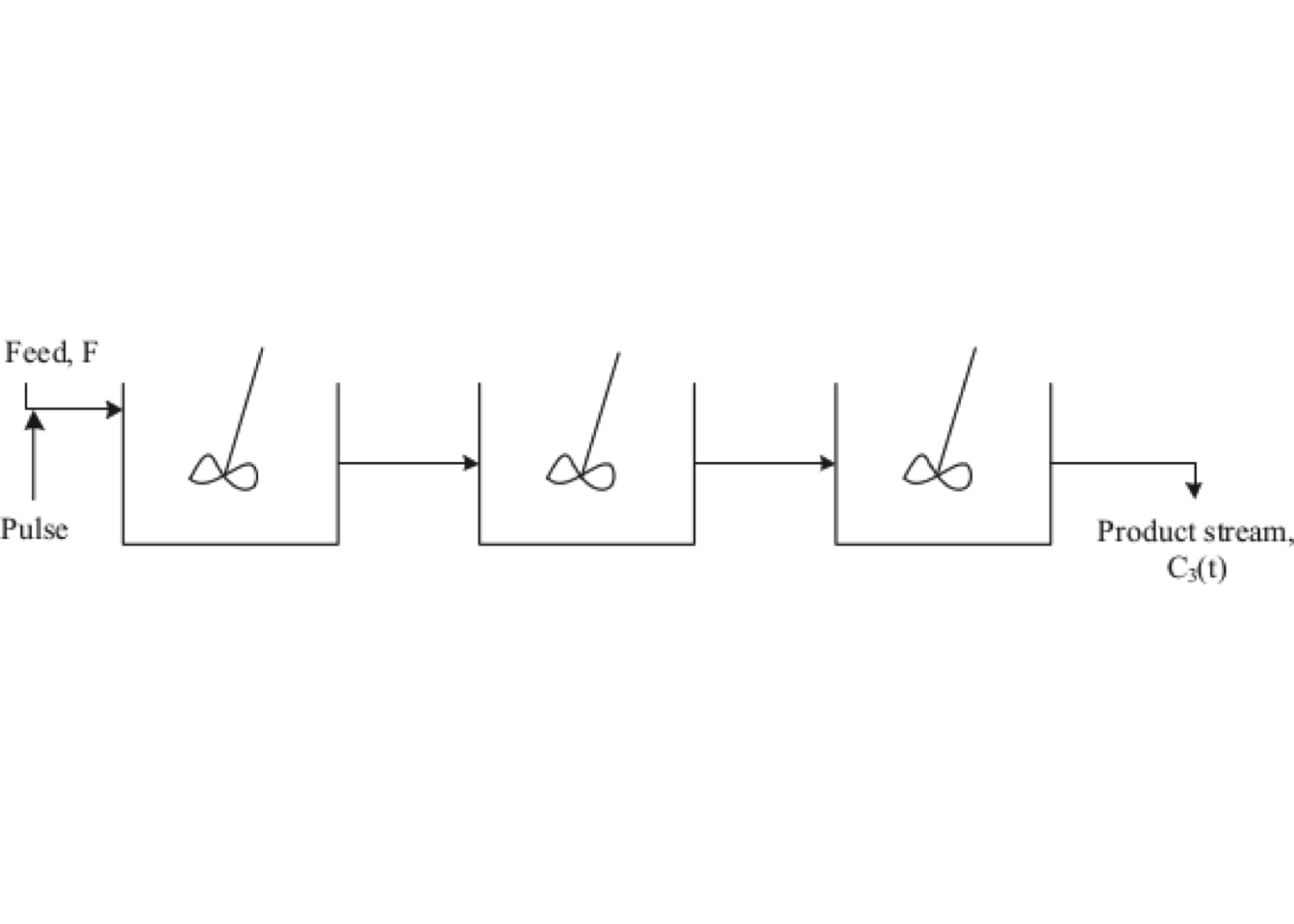
Figure 5.7: The tanks-in-series model uses a number of equally sized CSTRs placed in series
Performing the mole balance on the third vessel and solving in a similar way give the outlet concentration with time from the third reactor. \[\begin{equation} C_3(t) = \frac{C_0}{2}\,{\left(\frac{t}{\overline{t}_3}\right)}^2\,\exp{\left(-\frac{t}{\overline{t}_3}\right)} \tag{5.18} \end{equation}\]
Therefore, generalizing this method to a series of \(N\) CSTRs gives the RTD for \(N\) CSTRs in series: \[\begin{equation} \frac{C(t)}{C(t_0)} = \frac{t^{N-1}}{(N-1)!\,\overline{t}_i^N}\,\exp{\left(-\frac{t}{\overline{t}_i}\right)} \end{equation}\] taking into account that \(\overline{t} = N \: \overline{t_i}\) then \[\begin{equation} \frac{C(t)}{C(t_0)} = \mathbf{C}(t) = \frac{t^{N}}{(N-1)!}\,\left(\frac{t}{\overline{t}}\right)^{N-1}\exp{\left(-N\frac{t}{\overline{t}}\right)} \tag{5.19} \end{equation}\]
Equation (5.19) could be expressed with normalized time using \(\mathbf{C}(t) = \overline{t}\,\mathbf{E}(t)\), leading to the normalized distribution function is: \[\begin{equation} \mathbf{E}_N(\theta) = \frac{N^N}{(N-1)!}\,\theta^{N-1}\,\exp{\left(-N\theta\right)} \tag{5.20} \end{equation}\] where, again, \(\theta = t/\overline{t}\).
Figure 5.8 illustrates the RTDs of various numbers of CSTRs in series. As \(N\) increases from 1, the spread of distribution decreases. Furthermore, when \(N>2\), the peak would be an infinitive height (behavior of a PFR).
The mathematical illustration is available on the following link
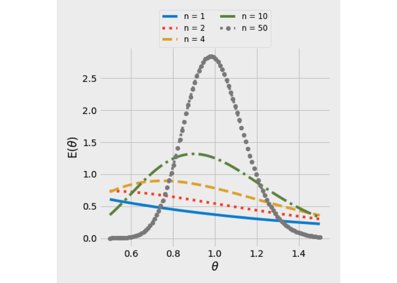
Figure 5.8: E(theta) curve using the tanks-in-series model
The cumulative RTD function \(\mathbf{F}{(\theta)}\) could be calculated from equation (5.20), for integral values of \(N\) \[\begin{equation} \mathbf{F}_N(\theta) = \int_0^\theta \mathbf{E}(\theta)\:d\theta \tag{5.21} \end{equation}\] The integral in equation (5.21) can be evaluated analytically: \[\begin{equation} \boxed{\mathbf{F}_N(\theta) = 1 - \exp \left(-N\,\theta\right)\,\sum\limits_{i=0}^{N-1}{\frac{(N\theta)^i}{i!}}} \tag{5.22} \end{equation}\]
The result for equation (5.21) is shown in Figure 5.9 for several values of \(N\). For \(N=1\), the result is that for a single CSTR, as \(N\) increases, the shape becomes more like a step function, corresponding to a plug-flow.
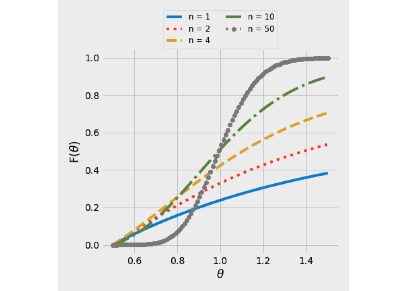
Figure 5.9: F(theta) curve using the tanks-in-series model
Finally, the washout function, \(\mathbf{W}{(\theta)}\), can be obtained from \(\mathbf{F}{(\theta)}\) \[\begin{equation*} \mathbf{W}{(\theta)} = 1 - \mathbf{F}{(\theta)} \end{equation*}\]
To utilize the tanks-in-series model, we need to determine the number of tanks that will give the same RTD as for the real system. This number may be obtained from the variance of RTD, which is given by the second moment about the mean: \[\begin{equation*} \sigma_{\theta}^2 = \int_0^\infty{{\left(\theta-1\right)}^2 \frac{\theta^{N-1}N^N}{(N-1)!}\,\exp{\left(-N\theta\right)}} = \int_{0}^{\infty} \theta ^2\mathbf{E}(\theta)\,d\theta - 1 \end{equation*}\] Solution of the integral equation gives the result \[\begin{equation*} \sigma_{\theta}^2 = \frac{\left(N+2-1\right)!}{N\cdot N!} - 1 = \frac{\left(N+1\right)!}{N\cdot N!} - 1 = \frac{1}{N} \end{equation*}\] The variance of the RTD is seen to be equal to the inverse of the number of tanks used. Therefore, if the RTD curve is known, the appropriated number of tanks in series to use may be calculated, so \[\begin{equation*} N = \frac{1}{\sigma_{\theta}^2} = \frac{\overline{t}^{ 2}}{\sigma^2} \end{equation*}\]
Exercise 5.2 (Estimate number of tanks based in Tanks-in-serie model) A step increase in the inlet trace A concentration, from 1.0 to 2.0 mmol/L, was used to determine the mixing pattern inside the fluidized-bed reactor. The response data were as follows:
| t (min) | C (mmol/L) | t (min) | C (mmol/L) |
|---|---|---|---|
| 0.0 | 1.000 | 30.0 | 1.410 |
| 5.0 | 1.005 | 45.0 | 1.610 |
| 10.0 | 1.020 | 60.0 | 1.770 |
| 15.0 | 1.060 | 90.0 | 1.920 |
| 20.0 | 1.200 | 120.0 | 1.960 |
Estimate values of \(N\) based on both central and backward differencing and determine which technique best describes the tracer outflow concentrations.
Solution
The solution is available on the next link
For each scenario, the equation (5.22) was applied to calculate the estimated \(\mathbf{F}(t)\), then based on Eq. (3.24), the output tracer concentration, \(C_{out}(t)\), may be calculated from \(\mathbf{F}(t)\).
Figure 5.10 shows the results of E(t) curve based on several numrical tecniques. On the other hand, Figure 5.11 shows the values of \(C_{out}(t)\) predicted using forward and central differencing technique, and based on a curve fitting approach. The last one provides a superior representation of the experimental data.
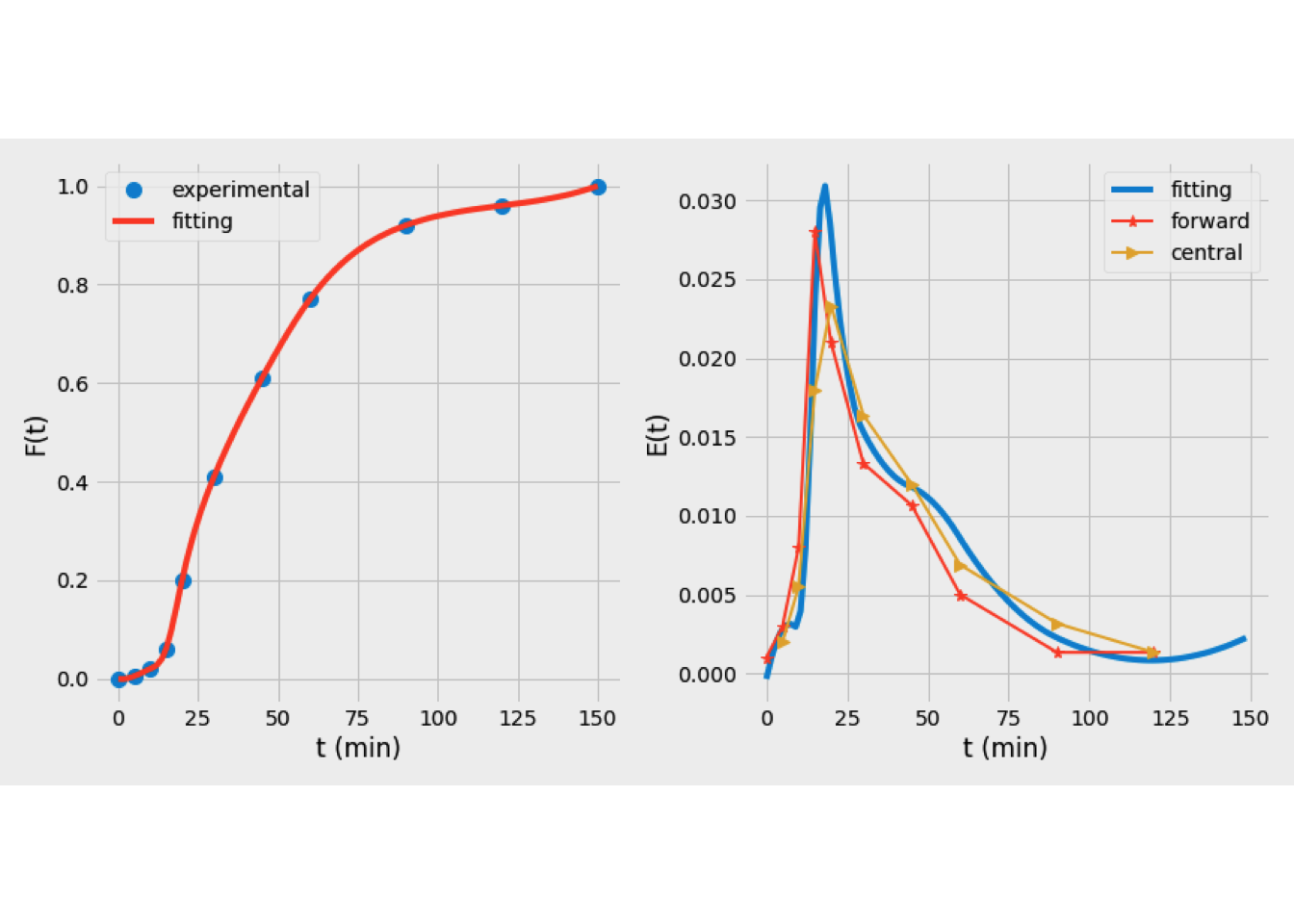
Figure 5.10: E(t) curves obtained based on several numerical tecniques applied to the tanks-in-series model
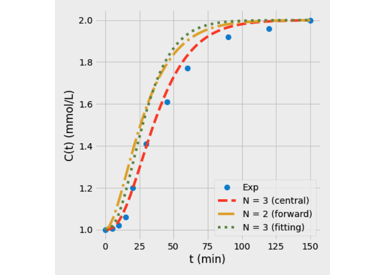
Figure 5.11: Selection of the best technique for the tanks-in-series model
The Dispersion Model
The dispersion model describes nonideal tubular reactors based on the assumption that exists an axial dispersion of the material, governed by Fick’s law diffusion-like, superimposed on the flow.
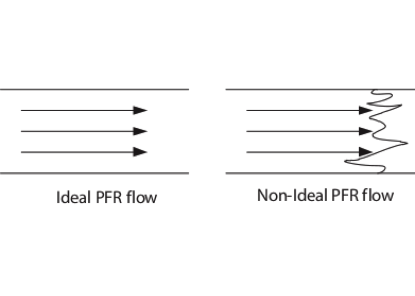
Figure 5.12: The dispersion model
Figure 5.12 shows a sketch of differences between velocity profiles between ideal PFR and actual flow. Fluctuations could be due to different flow and molecular velocities and turbulent diffusion. Although radial dispersion may also be significant, we consider only axial dispersion.
In considering axial dispersion as diffusive flow, it is assumed that Fick’s first law applies, with the effective diffusion coefficient replaced by an axial dispersion coefficient, \(D_L\). Thus, for unsteady-state behavior concerning a species \(T\) (tracer), the molar flux (\(N_T\)) of \(T\) at an axial position \(x\) is
\[\begin{equation*} N_T = - D_L \frac{\partial C_T(x,t)}{\partial x} \end{equation*}\] where \(C_T(x,t)\) is the concentration of \(T\).
Consider a material balance for \(T\) around the differential control volume shown in Figure 5.13.
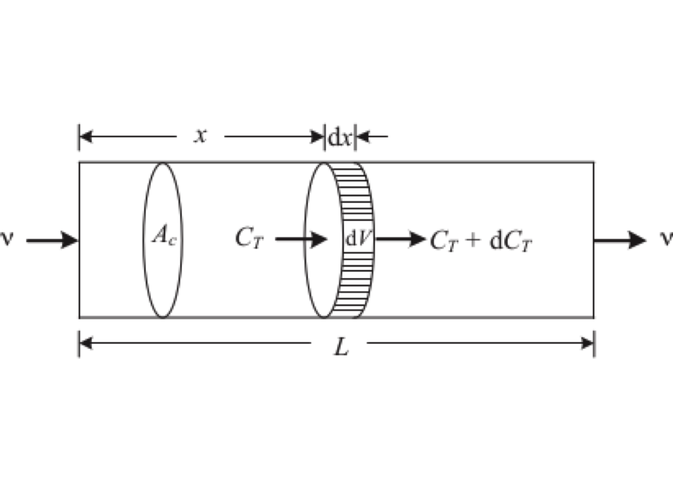
Figure 5.13: Control volume for continuity equation for axial dispersion
We assume steady flow overall, but not for tracer (\(T\)); there is no place.
Under those assumptions, with \(C_T \equiv C_T(x,t)\), \(A_c\) and \(D_L\) constant, for the transient flow of a non-reacting tracer, the mole balance equation is
\[\begin{equation} A_c\,\nu\,C_T - D_L\,A_c\,\frac{\partial C_T}{\partial x} - A_c\left[\nu C_T + \frac{\partial \left(\nu\,C_T\right)}{\partial x}\right] + D_L\,A_c\left[\frac{\partial C_T}{\partial x} + \frac{\partial}{\partial x} \left(\frac{\partial C_T}{\partial x}\right)\,dx\right] = A_c\,\frac{\partial C_T}{\partial t}\,dx \tag{5.23} \end{equation}\] where \(\nu\) is the average axial velocity (\(m/s\)), \(D_L\) is the axial dispersion coefficient, (\(m^2/s\)).
If system is density-constant and \(\nu\) is constant, the equation (5.23) becomes to \[\begin{equation} - D_L\,\frac{\partial^2 C_T}{\partial x^2} + \nu\,\frac{\partial C_T}{\partial x} = \frac{\partial C_T}{\partial t} \tag{5.24} \end{equation}\] If we know the boundary conditions of the problem, solving this equation, we get the profile of tracer concentration vs. time.
Equation (5.24) can be made dimensionless by defining the following scaling factors: \[\begin{equation*} z = \frac{x}{L}; \qquad \theta = \frac{t}{\overline{t}} = t\,\frac{\nu}{L} \qquad C^\ast = \frac{C_T}{C_0} \end{equation*}\] Here \(C_0\) is usually taken as the maximum concentration in the system.
\[\begin{equation} \frac{\partial C^\ast}{\partial \theta} = \left(\frac{D_L}{\nu \, L}\right) \frac{\partial ^2 C^\ast}{\partial z^2} -\frac{\partial C^\ast}{\partial z} \tag{5.25} \end{equation}\]
and \(D_L/(\nu\,L)\) is named the dispersion number, when \[\begin{align*} &\frac{D_L}{\nu\,L} \to 0 && \rightarrow &&\quad \text{large dispersion, hence well-mixed flow} &&\\ &\frac{D_L}{\nu\,L} \to \infty && \rightarrow &&\quad \text{negligible dispersion, hence plug flow}&& \end{align*}\]
We also have a dimensionless group, denoted Pe, which is called Peclet number based on vessel length. The physical interpretation is that it represents the ratio of convective flux to diffusive flux: \[\begin{equation*} \text{Pe} = \frac{\nu\,L}{D_L} \equiv \frac{\nu\,C_T}{D_L(C_T/L)} = \frac{\text{rate of transport by convection}}{\text{rate of transport by diffusion or dispersion}} \end{equation*}\]
So, we see that \[\begin{equation} \frac{\partial C^\ast}{\partial \theta} = \frac{1}{\text{Pe}}\frac{\partial ^2 C^\ast}{\partial z^2} -\frac{\partial C^\ast}{\partial z} \tag{5.26} \end{equation}\]
Now, the results of solutions of Eq. (5.26) will depend on the choice of boundary conditions at inlet \((z = 0)\) and outlet \((z = 1)\). There are several possibilities concerning ‘’closed’’ and ‘’open’’ vessels, which do not necessarily satisfy actual positions.
When the flow is undisturbed as it passes the entrance and exit boundaries, we will call this the open boundary condition. While, when we have plug flow outside the vessel up to the boundaries, we call this the closed boundary condition. There are up to four combinations of boundaries, closed-closed, open-open, or mixed, based on previous conditions. Figure 5.14 illustrates the closed and open extremes.
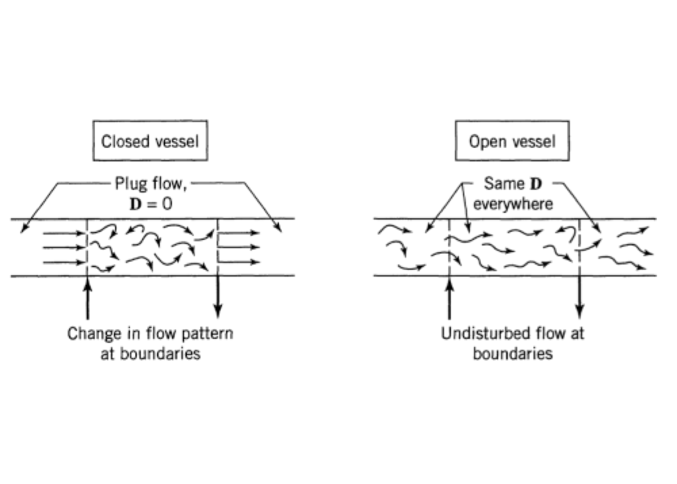
Figure 5.14: Boundary conditions used with dispersion model
For closed vessels, the flow conditions are illustrated schematically in Figure 5.15. \(D_L=0\), or \(Pe=\infty\) characterizes a plug-flow upstream of the vessel inlet. Since flow inside the vessel is dispersed, and the pulse injection is at inlet \((z=0)\), will have a \(C_T\) discontinuity across the inlet. In contrast, a continuity on CT across the outlet \((z=1)\) is usually assumed, even though downstream flow \((z>1)\) is plug-flow.
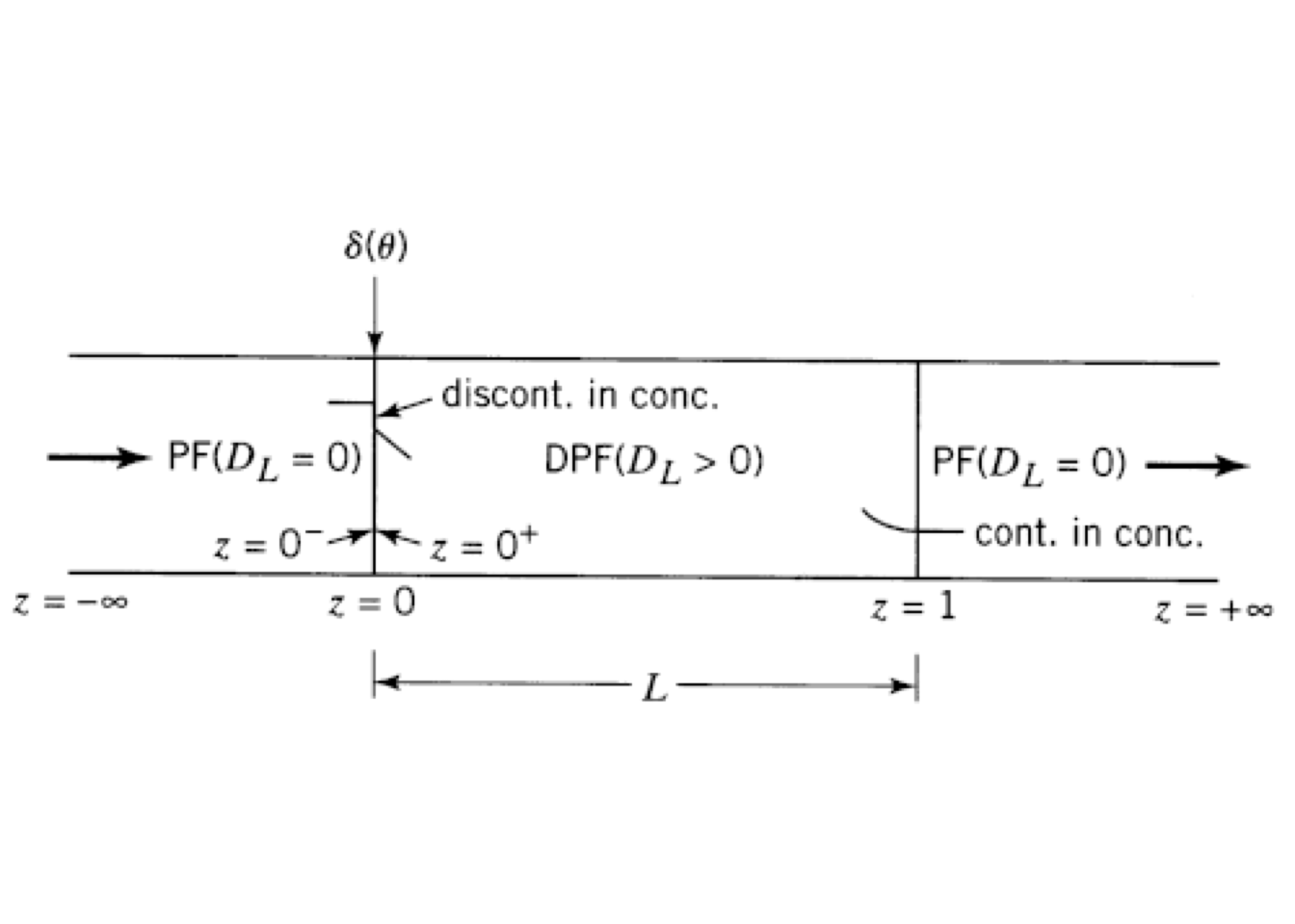
Figure 5.15: Flow conditions for closed-closed vessel
In this course, we only deal with a closed-closed case which is illustrated in Figure 5.15. Danckwerts formulated the closed configuration, and it means that there is no dispersion before \(z=0\) and after \(z=1\).
The equation (5.26) is a second-order boundary value problem requires two boundary conditions. If the system is taken as a closed system, the dimensionless boundary conditions are: \[\begin{align}\label{ec:004_046} &C_\text{in}^\ast = C^\ast-\frac{1}{\text{Pe}}\,\frac{\partial C^\ast}{\partial z} && \text{at } z = 0 && \qquad\\ & \frac{\partial C^\ast}{\partial z} = 0 &&\text{at } z = 1 && \qquad \tag{5.27} \end{align}\] Additionally, the system requires an initial condition: \[\begin{align} &C^\ast = 1 &&\text{at } \theta = 0, \text{ and } z = 0 && \qquad\\ &C^\ast = 0 &&\text{at } \theta = 0, \text{ and } 0 < z \leq 1 && \qquad \tag{5.28} \end{align}\]
An analytical solution to equation (5.26) with these boundary conditions is given by Otake and Kunigita (1598), but is rather complex, and it was omitted it here. However, moments and relatively simple an are given by: \[\begin{gather} \overline{\theta} = 1 \\ \sigma_\theta^2 = \frac{2}{\text{Pe}^2}\left(\text{Pe}-1+\exp(-\text{Pe})\right) \tag{5.29} \end{gather}\] An approximate closed form solutions for Pe > 50: \[\begin{gather*} \mathbf{F}(\theta) = \frac{1}{2} \left[1 - \text{erf}\left(\frac{1-\theta}{\sqrt{\theta}}\sqrt{\frac{\text{Pe}}{4}}\right)\right] \\ \mathbf{E}(\theta) = \frac{\exp\left(-\text{Pe}(1-\theta^2)/4\right)}{\sqrt{4\,\pi/\text{Pe}}} \end{gather*}\] where \(\text{erf}\) is the error function.
As a practical matter, these mathematical complexities should probably not be taken too literally since the precise conditions at the boundaries of actual equipment cannot usually be precisely defined in any event.
Where to get the dispersion coefficient?
- Experimental determination by analyzing pulse response. The Peclet number can be found experimentally using a pulse injection into the tube inlet and finding the RTD function. The Peclet number depends on the variance of the normalized RTD function:
\[\begin{equation} \sigma^2_{\theta} = \frac{2}{\text{Pe}} - \frac{2}{\text{Pe}^2}\left[1 - \exp(-\text{Pe})\right] \tag{5.30} \end{equation}\]
- Calculation from correlations. \[\begin{align*} & \frac{1}{\text{Pe}_R} = \frac{1}{Re \cdot Sc} + \frac{Re \cdot Sc}{192} && \text{ For } 1<Re< 2000 \text{ and } 0.23 < Sc < 1000\\ & \frac{1}{\text{Pe}_R} = \frac{3\cdot 10^7}{Re^{2.1}} + \frac{1.35}{Re^{1/8}} && \text{ For } Re > 2000 \end{align*}\] where
\[\begin{align*} &\text{Pe}_R = \frac{wd}{D} &&: \text{Peclet number in tube} &&\quad \\ &Re = \frac{wd}{\nu} &&:\text{Reynolds number} &&\quad \\ &Sc = \frac{\nu}{D_m} &&: \text{Schmidt number} &&\quad \end{align*}\]
Exercise 5.3 (Comparison in conversion calculation for a non-ideal flow reactor) For a reaction
\[\begin{equation} A \rightarrow B; \qquad r_A = -k\,C_A; \quad k = 0.25 \text{ min}^{-1} \end{equation}\]
Compare final conversions based on:
- axial dispersion model with closed vessel approximations.
- tanks in series model, and
- ideal PFR model.
| t (min) | C (g/m3) | t (min) | C (g/m3) |
|---|---|---|---|
| 1.00 | 1.000 | 7.00 | 4.000 |
| 5.00 | 2.000 | 8.00 | 4.000 |
| 3.00 | 8.000 | 9.00 | 2.200 |
| 4.00 | 10.00 | 10.0 | 1.500 |
| 5.00 | 8.000 | 12.0 | 0.600 |
| 6.00 | 6.000 | 14.0 | 0.000 |
Solution
The solution is available on the next link
Based on the axial dispersion model. We need to find the Pe number that is following RTD data.
In this case, we calculated from experimental data, the RTD curve, mean time and its variance. Then, the Eq. (5.30) was solved: \[\begin{equation*} \sigma^2_{\theta} = \frac{\sigma^2}{\overline{t}^2} = \frac{2}{\text{Pe}} - \frac{2}{\text{Pe}^2}\left[1 - \exp(-\text{Pe})\right] \Rightarrow Pe = 8.007 \end{equation*}\]
When a chemical reaction is included in the dispersion model, a numerical solution is usually required for the resulting differential equation. so, based on the reactions and considering a simple power-law rate expression, the mole balance of A is written as
\[\begin{equation*} D_L\frac{\partial^2 C_A}{\partial x^2} - \nu \, \frac{\partial C_A}{\partial x} - (k\,C_A^{\,n}) = 0 \end{equation*}\]
Which it could be written in dimensionless variables as: \[\begin{equation*} \frac{1}{\text{Pe}}\frac{\partial^2 C_A}{\partial z^2} - \nu \, \frac{\partial C_A}{\partial z} - (k\,\overline{t}\,C_A^{\,n}) = 0 \end{equation*}\]
And, in terms of the fractional conversion \[\begin{equation*} \frac{1}{\text{Pe}}\frac{\partial^2 X_A}{\partial z^2} - \frac{\partial X_A}{\partial z} - k\,\overline{t}\,C_{A0}^{\,n-1}{\left(1-X_A\right)}^n = 0 \end{equation*}\]
The fractional conversion is therefore governed by the magnitude of three dimensionless groups, Pe, \(n\), and \(k\overline{t}\,C_{A0}^{n-1}\). There is an analytical solution to this equation only for a first-order reaction: \[\begin{equation*} \frac{C_A}{C_{A0}} = 1 - X_A = \frac{4\,a\exp{\left(\text{Pe}/2\right)}}{{\left(1+a\right)}^2 \exp {\left(a\,\text{Pe}/2\right) }- {\left(1-a\right)}^2 \exp{\left(-a\,\text{Pe}/2\right)}} \end{equation*}\] where \[\begin{equation*} a = {\left(1 + \frac{4\,k\,\overline{t}}{\text{Pe}}\right)}^{0.5} \end{equation*}\] Solving this equation \(X_A = 0.6826\)
For calculating the fractional conversion based in TIS model, it is necessary to find de number of reactor that is in accordance with given RTD data. \[\begin{equation*} \text{number of reactors } = \frac{\overline{t}}{\sigma^2} = 4.4 \end{equation*}\] Then the conversion is \[\begin{equation*} X_A = 1 - \frac{C_{AN}}{C_{A0}} = 1 - \frac{1}{\left(1+k\,\overline{t}/N\right)^N} = 0.6736 \end{equation*}\]
For an ideal PFR. The fractional conversion is: \[\begin{equation*} X_A = 1 - \exp(-k\,\overline{t}) = 0.7253 \end{equation*}\]
In summary, why is it relevant to perform an analysis of RTDs?
This approach can ease the following tasks: 1. Diagnostics of problems in reactor operations. 2. Design of unit operations. 3. Predictions of conversion and effluent concentrations.
We have studied models of several simple, partially mixed reactors. These are shown in Figure 5.16 for increasing back mixing.
![Residence time distributions for the nonideal reactors. [@schmidt1998]](ebook_notes_5314_files/figure-html/fig004022-1.png)
Figure 5.16: Residence time distributions for the nonideal reactors. (Schmidt 1998)