Chapter 4 Applications for RTD functions

As it was said before, RTD provides a measure of macroscopic mixing; therefore, it could be helpful as a tool for:

1. detecting and characterizing flow behavior.
2. estimating of values of parameters for nonideal flow models.
3. assessment of the performance of a vessel as a reactor.

4.1 RTD functions for ideal reactors

\(\mathbf{F}(t)\) fits the behavior either when \(N\) particles are injected individually at different times to a steady-state reactor or if they are entered all at once to the reactor as \(\mathbf{F}(t)\) represents the volume fraction of the fluid leaving the reactor, which resided in the system over a time of \(t\) or less.

Plug Flow Reactor (PFR)

In this reactor, there is not back mixing. Hence, every fluid element has the same mean residence time \(\overline{t}\) (or \(\tau\)). This corresponding to a pulse tracer entering the reactor at time \(t=0\) during an infinitesimally short time and does not mix with fluid elements running ahead or behind it within the reactor.

The flow pattern in PFR could be represented in terms of the Dirac delta function \(\left( \delta \left(t - \overline{t} \right)\right)\).The Dirac delta function is a generalized function, on the real number line that is zero everywhere except at zero, where it is infinite:

\[\begin{equation*} \delta \left(t - \overline{t} \right) = \left \{ \begin{aligned} & \infty && t = \overline{t} \\ & 0 && t \neq \overline{t} \end{aligned} \right. \end{equation*}\]

Therefore, the normalized RTD function is written down in terms of Dirac “delta-function’’ \[\begin{equation} \mathbf{E}(t) = \delta (t - \overline{t} ) = \left \{ \begin{aligned} & \infty \text{ when } t = \overline{t} \\ & 0 \text{ when } t \neq \overline{t} \end{aligned} \right. \tag{4.1} \end{equation}\]

The integral of Dirac \(\delta\)-function is given as:

\[\begin{equation*} \int_a^b \delta {\left(t-\overline{t}\right)} \, f(t) dt = \left \{ \begin{aligned} & f(\overline{t}) \text{ when } a < \overline{t} < b \\ & 0 \text{ when } a > \overline{t} > b \end{aligned} \right. \end{equation*}\] where \(a\) and \(b\) are any constant.

Therefore, \[ \mathbf{F}(t) = \left \{ \begin{aligned} & 0 \text{ when } 0 < t < \overline{t} \\ & 1 \text{ when } t \geq \overline{t} \end{aligned} \right. \]

The moments of the normalized distribution all equal one, while the central moments equal zero.

Continuous Stirred Tank Reactor (CSTR)

An ideal CSTR implies that as soon as a fluid element (or pulse of tracer) is injected into the reactor, it distributes itself uniformly throughout the reaction zone. In “ideal’’ CSTRs, the exit stream is assumed to have the same composition as the reaction mixture within the reaction zone.

It follows that the exit stream will have the highest possible concentration of material from the tagged fluid element (or pulse tracer) at the outset of the experiment (i.e., \(t =0\)). After that, the tracer concentration in the main reactor would be diluted with the inlet stream, and the concentration of tracer in the exit stream would be expected to decay to zero gradually.

The RTD for a CSTR can be easily analyzed using a pulse injection. Assume, in the first instance, that the inlet stream to the vessel contains a concentration of the tracer equals to \(C_{TR,0}\), given by

\[\begin{equation} C_{TR,0} = \frac{N_{TR}}{V_R} \tag{4.2} \end{equation}\]

The decay of tracer concentration in the reactor is an unsteady state process given by, \[\begin{equation} -\upsilon\,C_{TR} = V_R\,\frac{dC_{TR}}{dt} \tag{4.3} \end{equation}\]

For a constant-density fluid, Eq. (4.3) could be rewritten as

\[\begin{equation} -\frac{\upsilon}{V_R}\,dt=-\frac{dt}{\overline{t}} = \frac{dC_{TR}}{C_{TR}} \tag{4.4} \end{equation}\]

Integrating Eq. (4.4) yields to: \[\begin{equation} C_{TR}(t) = C_{TR,0}\,\exp{\left(-\frac{t}{\overline{t}}\right)} \tag{4.5} \end{equation}\]

Now, substituting Eq. (4.5) into Eq. (3.25) \[\begin{equation} \mathbf{W}(t) = \frac{C_{TR}(t) - C_{TR}(\infty)}{C_{TR,0} - C_{TR}(\infty)} = \cfrac{C_{TR,0}\,\exp{\left(-\cfrac{t}{\overline{t}}\right)} }{C_{TR,0}} = \exp{\left(-\frac{t}{\overline{t}}\right)} \tag{4.6} \end{equation}\]

And, the RTD function is obtained by differentiation: \[\begin{equation} \mathbf{E}(t) = -\frac{d\,\mathbf{W}(t)}{dt} =\frac{1}{\overline{t}} \exp{\left(-\frac{t}{\overline{t}}\right)}\equiv \frac{C(t)}{\displaystyle\int_0^\infty C(t)\, dt} \tag{4.7} \end{equation}\]

The RTD decays exponentially with time. However, the area under the curve is always equal to unity because of the normalization. The typical residence time distribution for a CSTR is presented in Figure 4.1

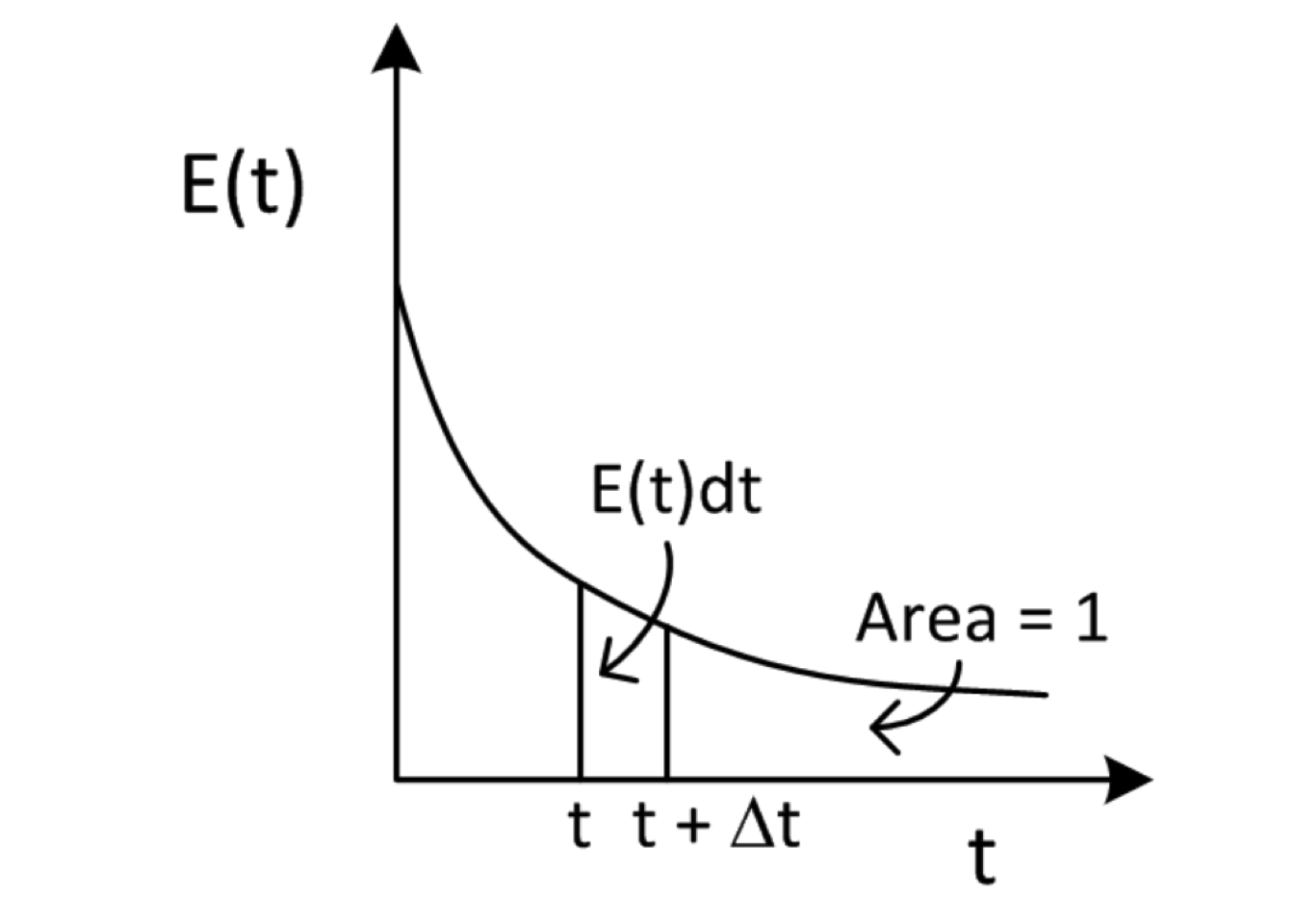
Figure 4.1: The residence time distribution E(t) in a CSTR and the time interval from t to t+dt

Other tracer experiments can be used to characterize flow patterns for non-ideal reactors. However, the input of a pulse or a step-change is commonly used in practice. Figures 4.2 and 4.3 summarize the exit concentration curves and the shapes of the \(\mathbf{E}(t)\) curves for a step change and input pulse of tracer, respectively.

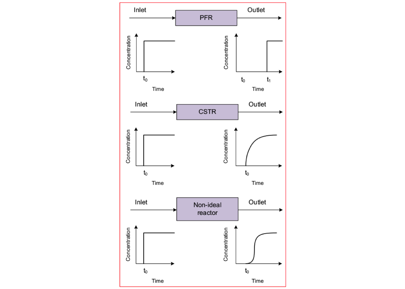
Figure 4.2: Response of tracer species during a step change experiment

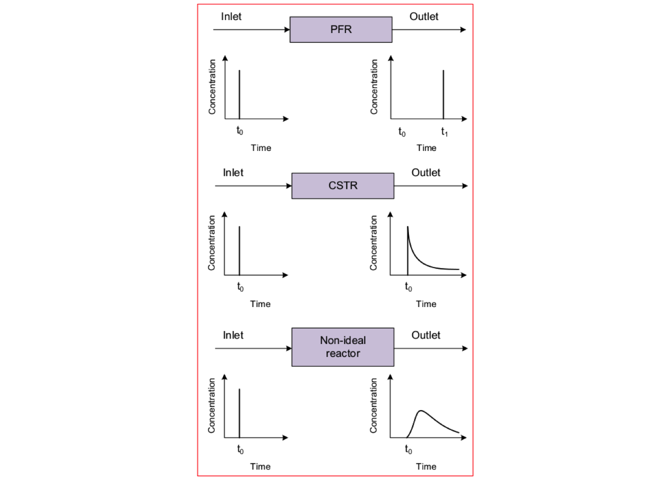
Figure 4.3: Response of tracer species during an input impulse experiment

4.2 RTD as diagnostic tool for characterizing flow behavior

The RTD curve can be used as a diagnostic method to determine the characteristics of reactor flow patterns. The methods of interpretation fall into two main categories:

1. processes with a relatively small degree of mixing, and
2. processes with significant deviations from ideal flow patterns, namely, dead space, bypassing, and general nonuniform regions.

Since these maldistributions can cause unpredictable conversion in reactors, they are usually detrimental to reactor operation.

Relatively Small Degree of Mixing

The age-distribution functions for flow patterns with a relatively small degree of mixing will have the general shapes shown in Figure 4.4

Figure 4.4: Effect of some features of nonideal flow on RTD. (Himmelblau and Bischoff 1968)

As is shown, the peak of the \(\mathbf{E}(\theta)\) curve will almost be at the mean holding time \(\theta = \overline{t}/\overline{t} = 1\), and \(\mathbf{I}(\theta)\) curve will have a value of about 0.5 at \(\theta = 1\). None of the curves will have excessively long tails and, in particular, the \(\mathbf{E}(\theta)\) will be almost symmetrical.

These features lead to the use of the type of description based on Gaussian curves, namely, the mean and the variance. \[\begin{align*} \text{mean} & = \mu_1 = \int_0^\infty \theta\,\mathbf{E}(\theta)\,d\theta = 1 \\ \text{variance} & = \sigma^2 = \int_0^\infty \left(\theta - \mu_1 \right)^2\,\mathbf{E}(\theta)\,d\theta \end{align*}\]

Detection of Dead Space

A process vessel may exhibit a region where fluid elements are retained for times of an order of magnitudes more significant than the mean residence time of the total fluid, what is called dead space. The existence of dead space is most easily verified from the characteristics of the \(\mathbf{E}(\theta)\) curve as shown in Figure 4.5. The \(\mathbf{E}(\theta)\) will have a very long tail indicating that fluid is held in the dead space.

Figure 4.5: Identification of the existence of dead space in a process vessel. (Himmelblau and Bischoff 1968)

The true mean residence time will be equal to the vessel volume divided by the flow rate \(\overline{t} = V/\upsilon\). However, the experimental data for times longer than \(\theta\) equal to 2 or 3 times mean residence time are seldom of sufficient accuracy to use in calculations. Thus, the calculated apparent mean residence time would be \[\begin{equation*} \overline{\theta}_a = \int_0^\theta \theta^\prime \, \mathbf{E}(\theta^\prime)\,d\theta^\prime, \qquad \theta \approx 2 \text{ or } 3 \end{equation*}\]

whereas the true mean would be \[\begin{align*} \theta & = \int_0^\infty \theta \, \mathbf{E}(\theta)\,d\theta = \int_0^\theta \theta^\prime \, \mathbf{E}(\theta^\prime)\,d\theta^\prime + \int_\theta^\infty \theta^\prime \, \mathbf{E}(\theta^\prime)\,d\theta^\prime = 1 \\ & = \overline{\theta}_a + \int_\theta^\infty \theta^\prime \, \mathbf{E}(\theta^\prime)\,d\theta^\prime = 1 \end{align*}\]

In presence of dead space, \(\overline{\theta}_a < 1\) or \(\overline{t}_a < \overline{t}\). The apparent mean gives a measure of the dead volumen of the vessel: \[\begin{equation*} \overline{t}_a = \frac{V_\text{active}}{\upsilon_\text{active}} = \frac{V - V_\text{dead}}{\upsilon_\text{active}} = \overline{t}\, \overline{\theta}_a \end{equation*}\]

This equation can be rewritten as \[\begin{align*} \frac{V_\text{dead}}{V} &= \frac{\upsilon_\text{active}}{V} \left(\frac{V}{\upsilon_\text{active}} - \overline{t}\overline{\theta}_a\right) \\ \frac{V_\text{dead}}{V} &= 1 - \overline{\theta}_a\,\overline{t}\,\frac{\upsilon_\text{active}}{V} \\ \frac{V_\text{dead}}{V} &= 1 - \overline{\theta}_a \left(\frac{\upsilon_\text{active}}{\upsilon} \right)\approx 1 - \overline{\theta}_a \end{align*}\]

One problem with using these relations is that they assume the true mean holding time, \(\overline{t}\), is known. Since it cannot be found from the trace curve (due to the inaccurate tail), it must be known independently and challenging to obtain.

Detection of Bypassing

If a portion of fluid spends one-tenth of the overall fluid’s mean residence time, this fluid can be said to bypass the vessel for all practical purposes. The \(\mathbf{E}(\theta)\) curve would then appear as in Figure 4.6.

Figure 4.6: Identification of the existence of bypassing in a process vessel. (Himmelblau and Bischoff 1968)

If there is a large amount of dead space or bypassing, the distinction between the two is not clear-cut but depends on which part of the fluid is considered the “major’’ part, a somewhat arbitrary assignment.

However, \(\mathbf{E}(\theta)\) can be used to detect dead space or bypassing (as discussed above). If the true mean holding time is not known, this curve cannot be used to determine dead space. Instead, the \(\mathbf{I}(\theta)\) curve must be used because it always has the same shape as regards the existence of maxima no matter what the time scale. Therefore, the most significant utility of the intensity function is to determine dead space from experimental data, especially if the true mean holding time is unknown.

Figure 4.7 summarizes the typical shapes of the \(\mathbf{E}(\theta)\) curve of (a) stagnation, (b) dispersion and (c) channeling or excessive bypassing.

Figure 4.7: Effect of some features of nonideal flow on RTD. (Missen, Mims, and Bradley 1999)

If large amounts of dead space of bypassing exist, it may not be worthwhile to try to construct a detailed mathematical model because the unit is sure to give poor performance. Thus, some modifications might be called for to eliminate the severe mixing problems.

In order to provide a better picture of the behavior of the distribution functions, a simple mathematical model will be considered that includes the possibility of having well-defined dead space and bypassing. The model consists of two parallel streams, each with a given number of perfectly mixed tanks in series as shown in Figure 4.8

Figure 4.8: Scheme of the mathematical representation. (Himmelblau and Bischoff 1968)

The RTD for this model with \(j\) stirred tanks in series is \[\begin{equation*} \mathbf{E}(t) = \frac{j^j}{\left(j-1\right)!} \frac{t^{j-1}}{\overline{t}}\exp\left(-\frac{j\,t}{\overline{t}}\right) \end{equation*}\] where \(\overline{t}\) is the mean residence time. If the equation is used for each branch of the model and weighted with respect to the amount of flow in the branch, the RTD for the entire model is: \[\begin{equation*} \mathbf{E}(t) = f\,\left(\frac{n^n}{\left(n-1\right)!} \frac{t^{n-1}}{\overline{t}_1}\exp\left(-\frac{n\,t}{\overline{t}_1}\right)\right) + \left(1-f\right)\,\left(\frac{m^m}{\left(m-1\right)!} \frac{t^{m-1}}{\overline{t}_2}\exp\left(-\frac{m\,t}{\overline{t}_2}\right)\right) \end{equation*}\] where \(f\) represents the fraction of flow to branch 1. The mean residence time is \[\begin{equation*} \overline{t} = f\, \overline{t}_1 + \left(1 - f\right)\, \overline{t}_2 \end{equation*}\]

Dimensionless variables based on the total mean residence time, \(\overline{t}\) can now be defined: \[\begin{equation*} \theta = \frac{t}{\overline{t}} \quad \alpha = \frac{\overline{t}_2}{\overline{t}_1} \quad \beta = f + \left(1 - f\right) \alpha \end{equation*}\]

Three situations were considered:

1. Fifteen tanks in each branch correspond to a relatively small amount of mixing in the branch.
2. Two tanks in each branch correspond to a large amount of mixing in the branch.
3. Four tanks in each branch correspond to a moderate amount of mixing in the branch.

Scenario 1. is shown in Figure 4.9. The rest of scenarios is available clicking on the next link

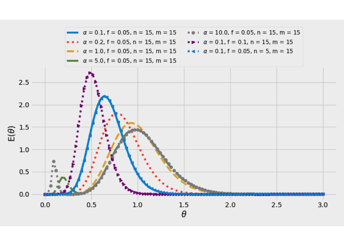
Figure 4.9: RTD curves for parallel stirred-tanks models.

References

Himmelblau, David D., and Kenneth B. Bischoff. 1968. Process Analysis and Simulation. John Wiley & Sons, INC.

Missen, Ronald, Charles Mims, and Saville. Bradley. 1999. Introduction to Chemical Reaction Engineering and Kinetics. John Wiley & Sons.